Welcome to the first post in our foundational statistics series! We live in a world overflowing with data—from website clicks and stock prices to sports scores and medical reports. But how do we make sense of it all? How do we distill millions of data points into a single, understandable story?
The answer lies in statistics, the art and science of learning from data.
This guide is your first step. We’ll start with the absolute basics, exploring the simple yet powerful tools we use to summarize information. By the end, you’ll have a rock-solid understanding of the three most fundamental concepts in descriptive statistics: the Mean, Median, and Mode.
What is Statistics, Anyway?
In the simplest terms, statistics is the practice of getting your head around data. It’s a collection of methods for collecting, analyzing, interpreting, and presenting information. Think of it as a detective’s toolkit for finding clues hidden within numbers.
Statistics can be broadly split into two main branches:
- Descriptive Statistics: This is all about summarizing and organizing data so we can easily understand it. If you have a massive spreadsheet of numbers, descriptive statistics help you describe it with a few key figures or graphs. Example: Calculating the average grade for a class.
- Inferential Statistics: This is where we play detective. We take a small piece of data (a sample) and use it to make an educated guess, or inference, about a much larger group (a population). Example: Surveying 1,000 voters to predict a national election outcome.
For today, our focus is on the descriptive side—learning how to tell the story of the data we already have.
The Heart of Your Data: Introducing Central Tendency
Imagine you’re asked to describe a dataset containing thousands of numbers. Reading them all out would be impossible. Instead, you’d likely try to find one single number that best represents the entire set.
This single, representative number is what we call a measure of central tendency.
Definition: Central Tendency A measure of central tendency is a single value that attempts to describe a set of data by identifying the central position within that set. It’s often called the “average” in everyday language.
It gives us a quick, digestible summary—a “typical” value that the other numbers cluster around. The three most common ways to measure this are the mean, median, and mode.
The Three Core Measures of “Average”
While we often use the word “average” casually, in statistics, it’s more precise to talk about the mean, median, and mode. Think of them as three different tools for the same job, each with its own strengths and weaknesses.
Let’s explore them with a simple dataset. Suppose we have the test scores of five students:
{1, 1, 2, 3, 4}
The Mean: The Familiar Arithmetic Average
This is the one you probably already know. When people talk about taking the “average,” they are almost always referring to the arithmetic mean.
The method is simple: add up all the values and divide by the number of values.
The formula looks like this:
Mean=Number of valuesSum of all values=n∑i=1nxi
Let’s apply it to our dataset: {1, 1, 2, 3, 4}.
- Sum the values: 1+1+2+3+4=11
- Count the number of values: There are 5 numbers.
- Divide the sum by the count: 5/11=2.2
So, the mean of our dataset is 2.2. This number gives us a sense of the central point that all the other numbers are balanced around.
The Median: The Middle Ground
The median is the value that sits in the exact middle of a dataset after it has been sorted in order from smallest to largest. It’s the true halfway point.
Calculating the median involves a simple two-step process:
- Sort your data from smallest to largest.
- Find the number in the very middle.
Using our dataset {1, 1, 2, 3, 4}, it’s already sorted. With five numbers, the middle one is easy to spot:
1, 1, 2, 3, 4
There are two values to its left and two to its right. The median is 2.
But what if you have an even number of values?
Let’s add a number to our set: {1, 1, 2, 3, 4, 4}. Now there are six values, and there’s no single middle number.
In this case, you take the two middle numbers, add them together, and calculate their mean.
1, 1, 2, 3, 4, 4
- The two middle numbers are 2 and 3.
- Take their mean: (2+3) / 2 = 2.5
The median of this new set is 2.5.
The Mode: The Most Popular Choice
The mode is the simplest of the three: it’s the value that appears most frequently in the dataset. Think “mode is most.”
Let’s look at our original set again: {1, 1, 2, 3, 4}.
Which number appears most often? The number 1 appears twice, while all others appear only once.
Therefore, the mode is 1.
Tip: What if there’s a tie? A dataset can have more than one mode.
{1, 1, 2, 3, 4, 4}: Here, both 1 and 4 appear twice. This dataset is bimodal (it has two modes).{1, 2, 3, 4, 5}: Here, no number repeats. This dataset has no mode.
The mode is especially useful for categorical data (like “most common car color”) but can be less reliable for numerical data if no numbers repeat.
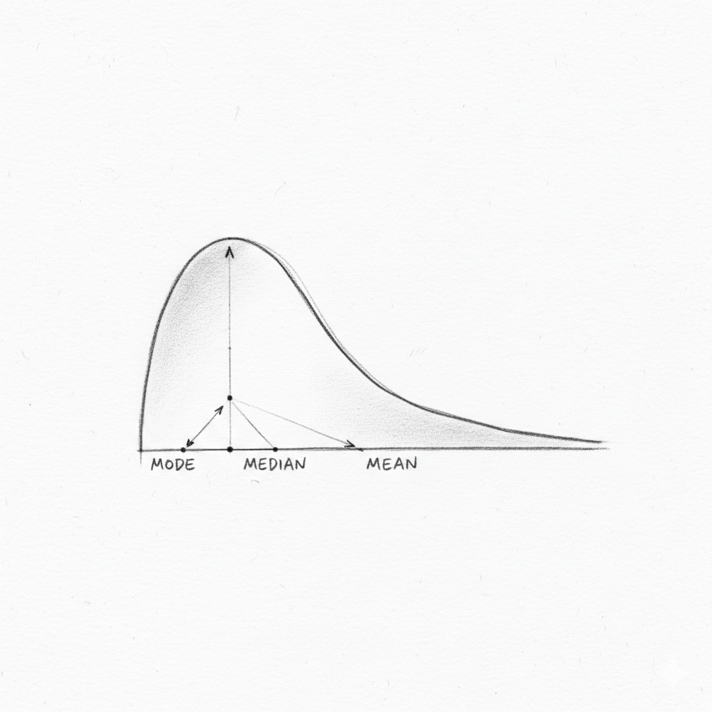
The Big Question: When Should You Use Mean vs. Median vs. Mode?
So, why do we need three different measures? Because a dataset can sometimes have “problem children”—numbers that are wildly different from the rest. These are called outliers.
The most important difference between the mean and the median is how they are affected by outliers.
Let’s imagine we’re analyzing the salaries at a small company with six employees. Their annual salaries are: {$50k, $52k, $55k, $58k, $60k, $500k}
That last salary, $500k, belongs to the CEO and is a clear outlier. Now, let’s calculate the mean and median to see what happens.
Calculating the Mean:
Mean=650+52+55+58+60+500=6775≈$129.17k
The mean salary is $129,170. If someone told you this was the “average” salary, you’d think the company pays extremely well. But does it really represent the typical employee’s earnings? Not really. Five out of six employees earn far less than that.
Calculating the Median: Our data is already sorted. Since we have an even number of values, we take the middle two:
$50k, $52k, $55k, $58k, $60k, $500k
Median= (55+58) / 2= $56.5k
The median salary is $56,500. This number is much more representative of what a typical employee at this company earns. It completely ignored the CEO’s outlier salary.
This leads to a crucial rule of thumb:
| Measure | Best for… | Weakness |
| Mean | Symmetrical data with no outliers. | Highly sensitive to outliers. |
| Median | Skewed data or data with outliers. | Can be less sensitive to small changes. |
| Mode | Categorical data or finding the most common item. | Can be ambiguous (bimodal/no mode). |
Key Takeaways
- Statistics is about summarizing and interpreting data.
- Central Tendency is a single value representing the “center” or “typical” value of a dataset.
- The Mean is the arithmetic average (sum/count). It’s powerful but easily skewed by outliers.
- The Median is the middle value of a sorted dataset. It’s robust and resists the pull of outliers.
- The Mode is the most frequent value. It’s great for identifying the most popular item.
- Choosing the right measure depends on your data. For skewed data (like salaries or house prices), the median is often a more truthful summary than the mean.
Frequently Asked Questions (FAQ)
1. What is the main difference between mean and median? The main difference is their sensitivity to outliers. The mean incorporates every value, so extreme values (outliers) can pull it significantly in their direction. The median only cares about the middle position, so it is not affected by outliers.
2. Can a dataset have more than one mode? Yes. If two or more values are tied for the most frequent occurrence, the dataset is called bimodal (two modes) or multimodal (many modes).
3. Why is the mean not always the best measure of central tendency? Because it can be misleading for skewed datasets. For example, the average house price in a neighborhood could be very high due to one mansion, while the median price would give a more accurate picture of what a typical house costs.
Leave a Reply